The book-to-market ratio (BM) is one of the most frequently calculated variables in accounting research and is usually used as a control variable in regressions. However, how to calculate it is a question I often asked when I started my PhD, as nobody defined it clearly in their papers. Should I use CEQ or SEQ, assets minus liabilities, or something else? This question becomes even more confusing when I realize that finance researchers often define the book value of equity differently from accounting researchers.
A related question is how to verify the basic accounting equation (A = L + E) using Compustat Annual (FUNDA) or Quarterly (FUNDQ) data? To answer this question, I checked the Compustat Manuals – Balancing Models – North American Company Data:
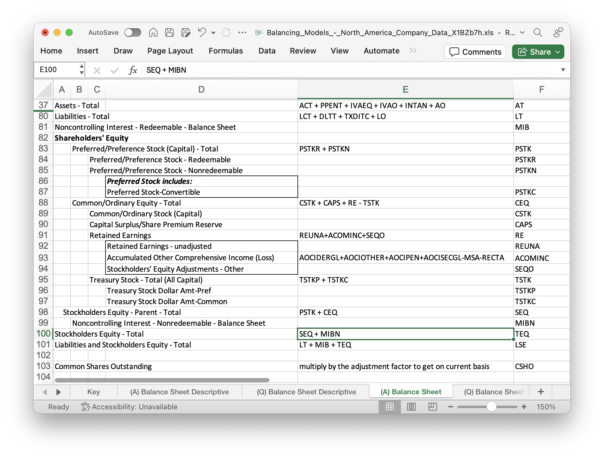
Therefore, the basic accounting equation is reflected in the following relationship:
AT = LSE
Or AT = LT + MIB + TEQ
The first equation can be verified using FUNDA data. However, the second equation holds true for only 42% of observations. Further investigation indicates that prior to FASB 160, LSE = LT + MIB + SEQ, while after FASB 160, LSE = LT + MIB + TEQ. That’s why the above second equation won’t hold true prior to FASB 160.
Returning to the initial question, BM = Book Value of Equity (BVE) / Market Value of Equity (MVE). When calculating MVE, we appear only able to use MVE = csho × prcc_f, where csho is the number of common shares outstanding, and prcc_f is the share price at the fiscal year-end. Therefore, MV will be the market value of common shares. To match this, it seems appropriate to define BVE as ceq(also common shares), and thus BM = ceq / (csho × prcc_f).
In contrast, in the sample code provided by WRDS to replicate Fama-Frech’s three factors, as well as in the Financial Ratios macro provided by WRDS, BVE = seq + txditc – pstk. The definitions of these variables can be found in the above figure. Although seq – pstk = ceq, I have no clue why txditc should be added. Perhaps finance researchers can shed light on this.